Q&A 17 How do you compare L1 and L2 regularization in regression models?
17.1 Explanation
Regularization is used to prevent overfitting by penalizing large model coefficients. Two common types are:
- L1 Regularization (Lasso): Adds a penalty equal to the absolute value of the magnitude of coefficients. This can shrink some coefficients exactly to zero, leading to feature selection.
- L2 Regularization (Ridge): Adds a penalty equal to the square of the magnitude of coefficients. This shrinks coefficients toward zero, but usually does not eliminate them entirely.
In practice:
- L1 is useful when you suspect some features are irrelevant.
- L2 is better when all features are likely relevant, but you want to reduce model complexity.
Let’s compare their effects on the Boston housing dataset.
17.2 Python Code
import pandas as pd
import matplotlib.pyplot as plt
from sklearn.linear_model import Ridge, Lasso
from sklearn.preprocessing import StandardScaler
from sklearn.model_selection import train_test_split

# Load and prepare data
df = pd.read_csv("data/boston_housing.csv")
X = df.drop("medv", axis=1)
y = df["medv"]

# Standardize features
scaler = StandardScaler()
X_scaled = scaler.fit_transform(X)

# Train-test split
X_train, X_test, y_train, y_test = train_test_split(X_scaled, y, test_size=0.3, random_state=42)

# Fit Ridge and Lasso
ridge = Ridge(alpha=1.0).fit(X_train, y_train)
lasso = Lasso(alpha=0.1).fit(X_train, y_train)

# Plot coefficients
plt.figure(figsize=(10, 5))
plt.plot(ridge.coef_, 'o-', label="Ridge (L2)")
plt.plot(lasso.coef_, 'x-', label="Lasso (L1)")
plt.xticks(range(X.shape[1]), X.columns, rotation=45)
plt.ylabel("Coefficient value")
plt.title("L1 vs. L2 Regularization Coefficients")
plt.legend()
plt.tight_layout()
plt.show()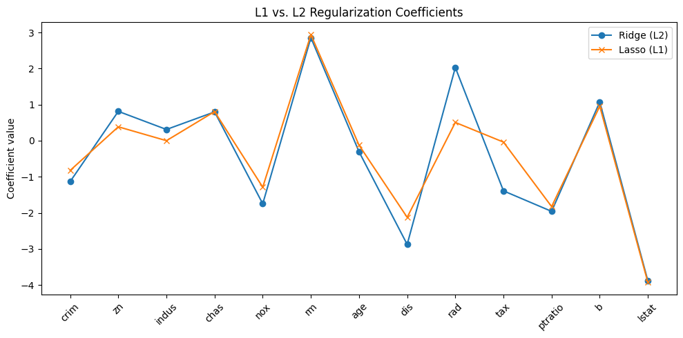
17.3 R Code
library(tidyverse)
library(glmnet)

# Load data
df <- read_csv("data/boston_housing.csv")
X <- df %>% select(-medv)
y <- df$medv

# Standardize
X_scaled <- scale(as.matrix(X))
y_vec <- as.numeric(y)

# Fit models
ridge_model <- glmnet(X_scaled, y_vec, alpha = 0)  # L2
lasso_model <- glmnet(X_scaled, y_vec, alpha = 1)  # L1

# Plot coefficients
plot(ridge_model, xvar = "lambda", label = TRUE, main = "Ridge (L2) Coefficients\n")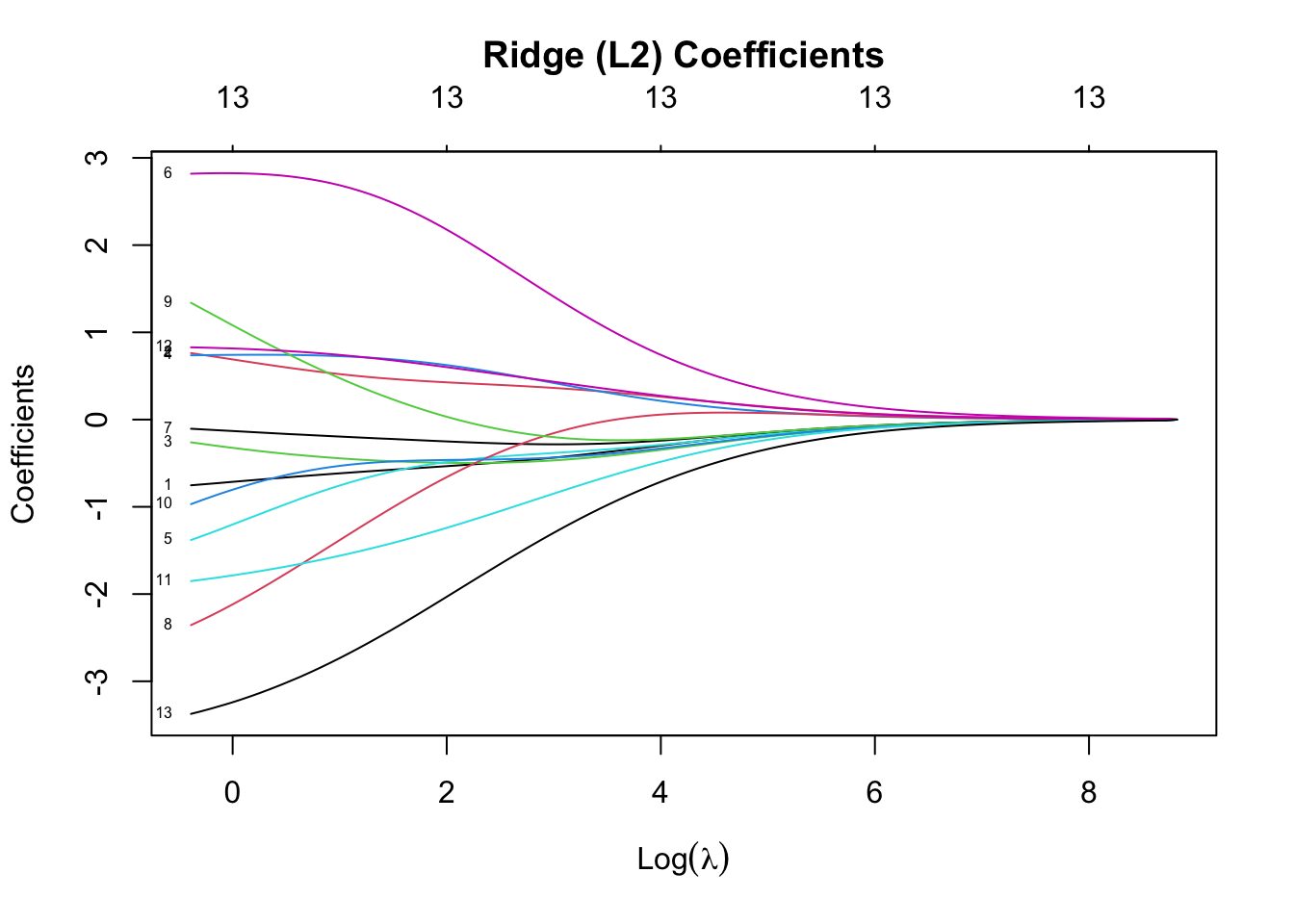
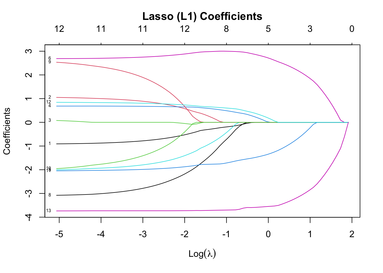
✅ Takeaway: L1 (Lasso) can eliminate irrelevant features by setting coefficients to zero. L2 (Ridge) shrinks all coefficients but retains all features. Try using ElasticNet for a combination of both!