Q&A 25 How do you compare multiple models and choose the best one?
25.1 Explanation
When working on a classification problem, it’s important to try multiple models and compare their performance using consistent metrics like accuracy, AUC, and ROC curves.
In this Q&A, we: - Use cross-validation to assess and compare model accuracy - Plot ROC curves to visualize how well each model distinguishes between classes - Summarize performance using both visual and numerical summaries
This helps us make an informed decision on which model best suits the task.
25.2 Python Code
# Compare classification models using CV and ROC in Python
import pandas as pd
import matplotlib.pyplot as plt
from sklearn.model_selection import cross_val_score, StratifiedKFold, train_test_split
from sklearn.metrics import roc_curve, roc_auc_score
from sklearn.preprocessing import LabelEncoder
from sklearn.linear_model import LogisticRegression
from sklearn.tree import DecisionTreeClassifier
from sklearn.ensemble import RandomForestClassifier, ExtraTreesClassifier
from sklearn.svm import SVC
from sklearn.naive_bayes import GaussianNB
from sklearn.discriminant_analysis import LinearDiscriminantAnalysis
from sklearn.neighbors import KNeighborsClassifier

# Load dataset
df = pd.read_csv("data/titanic.csv")

# Prepare features and target
df = df.dropna(subset=["Age", "Fare", "Embarked", "Sex", "Survived"])
# X = df[["Pclass", "Age", "Fare"]]
# Make a copy to avoid SettingWithCopyWarning
X = df[["Pclass", "Age", "Fare"]].copy()

X["Sex"] = LabelEncoder().fit_transform(df["Sex"])
X["Embarked"] = LabelEncoder().fit_transform(df["Embarked"])
y = df["Survived"]

# Split for final ROC comparison
X_train, X_test, y_train, y_test = train_test_split(X, y, test_size=0.3, random_state=42)

# Define models
models = [
    ("LR", LogisticRegression(solver="liblinear")),
    ("LDA", LinearDiscriminantAnalysis()),
    ("KNN", KNeighborsClassifier()),
    ("CART", DecisionTreeClassifier()),
    ("NB", GaussianNB()),
    ("EXT", ExtraTreesClassifier(n_estimators=10)),
    ("SVM", SVC(probability=True, gamma="auto", random_state=42)),
    ("RF", RandomForestClassifier(max_depth=2, random_state=42))
]

# Cross-validation
cv_results = []
names = []
for name, model in models:
    kfold = StratifiedKFold(n_splits=10, shuffle=True, random_state=1)
    scores = cross_val_score(model, X_train, y_train, cv=kfold, scoring="accuracy")
    cv_results.append(scores)
    names.append(name)
    print(f"{name}: {scores.mean():.4f} ({scores.std():.4f})")

# Accuracy boxplot
plt.boxplot(cv_results, tick_labels=names)
plt.title("Model Accuracy Comparison")
plt.xlabel("Algorithm")
plt.ylabel("Cross-Validated Accuracy")
plt.show()
LR: 0.7934 (0.0561)
LDA: 0.7994 (0.0516)
KNN: 0.6929 (0.0482)
CART: 0.7487 (0.0631)
NB: 0.7831 (0.0454)
EXT: 0.7871 (0.0349)


SVM: 0.6547 (0.0348)


RF: 0.7932 (0.0429)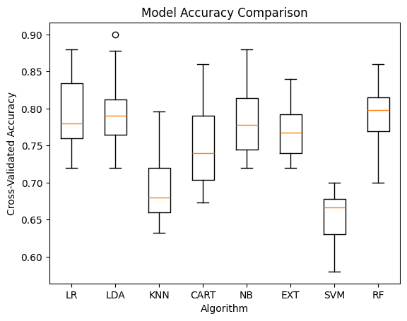
# ROC Curves
plt.figure(figsize=(8, 8))
for name, model in models:
    model.fit(X_train, y_train)
    probs = model.predict_proba(X_test)[:, 1]
    fpr, tpr, _ = roc_curve(y_test, probs)
    auc = roc_auc_score(y_test, probs)
    plt.plot(fpr, tpr, label=f"{name} (AUC = {auc:.4f})")

plt.plot([0, 1], [0, 1], linestyle="--", color="gray")
plt.xlabel("False Positive Rate")
plt.ylabel("True Positive Rate")
plt.title("ROC Curves for Classification Models")
plt.legend()
plt.show()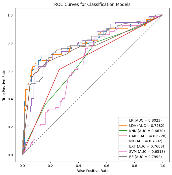
25.3 R Code
# Load required packages
library(tidyverse)
library(caret)
library(ggplot2)
library(randomForest)
library(e1071)
library(MASS)
library(class)
library(naivebayes)
library(rpart)

# Load dataset
df <- read_csv("data/titanic.csv") %>%
  filter(!is.na(Age), !is.na(Fare), !is.na(Sex), !is.na(Embarked), !is.na(Survived)) %>%
  mutate(
    Sex = factor(Sex),
    Embarked = factor(Embarked),
    Survived = factor(Survived)
  )

# Feature selection
df <- df %>% dplyr::select(Survived, Pclass, Age, Fare, Sex, Embarked)

# Train-test split
set.seed(42)
train_index <- createDataPartition(df$Survived, p = 0.7, list = FALSE)
train_data <- df[train_index, ]
test_data  <- df[-train_index, ]

# Train control for 10-fold cross-validation
ctrl <- trainControl(method = "cv", number = 10)

# Define models
models <- list(
  LR   = train(Survived ~ ., data = train_data, method = "glm", family = "binomial", trControl = ctrl),
  LDA  = train(Survived ~ ., data = train_data, method = "lda", trControl = ctrl),
  KNN  = train(Survived ~ ., data = train_data, method = "knn", trControl = ctrl),
  CART = train(Survived ~ ., data = train_data, method = "rpart", trControl = ctrl),
  NB   = train(Survived ~ ., data = train_data, method = "naive_bayes", trControl = ctrl),
  RF   = train(Survived ~ ., data = train_data, method = "rf", trControl = ctrl),
  SVM  = train(Survived ~ ., data = train_data, method = "svmRadial", trControl = ctrl)
)

# Collect resamples
res <- resamples(models)
summary(res)
Call:
summary.resamples(object = res)

Models: LR, LDA, KNN, CART, NB, RF, SVM
Number of resamples: 10

Accuracy
          Min.   1st Qu.    Median      Mean   3rd Qu.      Max. NA's
LR   0.6600000 0.7551020 0.7800000 0.7775302 0.8000000 0.8800000    0
LDA  0.6800000 0.7685294 0.7900000 0.7875726 0.8275510 0.8600000    0
KNN  0.6200000 0.6751020 0.7000000 0.6934062 0.7200000 0.7551020    0
CART 0.7058824 0.8000000 0.8000000 0.7876903 0.8000000 0.8367347    0
NB   0.7000000 0.7200000 0.7677551 0.7595758 0.7950000 0.8163265    0
RF   0.7400000 0.7810784 0.8100000 0.8256967 0.8793878 0.9200000    0
SVM  0.7600000 0.7800000 0.7800000 0.7935366 0.8190816 0.8235294    0

Kappa
          Min.   1st Qu.    Median      Mean   3rd Qu.      Max. NA's
LR   0.3089431 0.4789297 0.5454545 0.5353782 0.5848643 0.7540984    0
LDA  0.3220339 0.5220779 0.5608629 0.5537322 0.6325020 0.7107438    0
KNN  0.2016807 0.3383328 0.3553381 0.3487235 0.3957337 0.4683544    0
CART 0.3884892 0.5574200 0.5762712 0.5491182 0.5838533 0.6455696    0
NB   0.4000000 0.4190574 0.5199541 0.5019963 0.5645708 0.6107679    0
RF   0.4036697 0.5320038 0.5958279 0.6224569 0.7495806 0.8305085    0
SVM  0.4736842 0.5066970 0.5293644 0.5482346 0.6008261 0.6165414    0
✅ Takeaway: Don’t rely on a single algorithm. By testing multiple models and comparing accuracy and AUC, you’ll make better, more informed decisions — especially in real-world datasets where one model rarely fits all.