Q&A 18 How do you visualize L1 vs. L2 regularization paths side by side in R?
18.1 Explanation
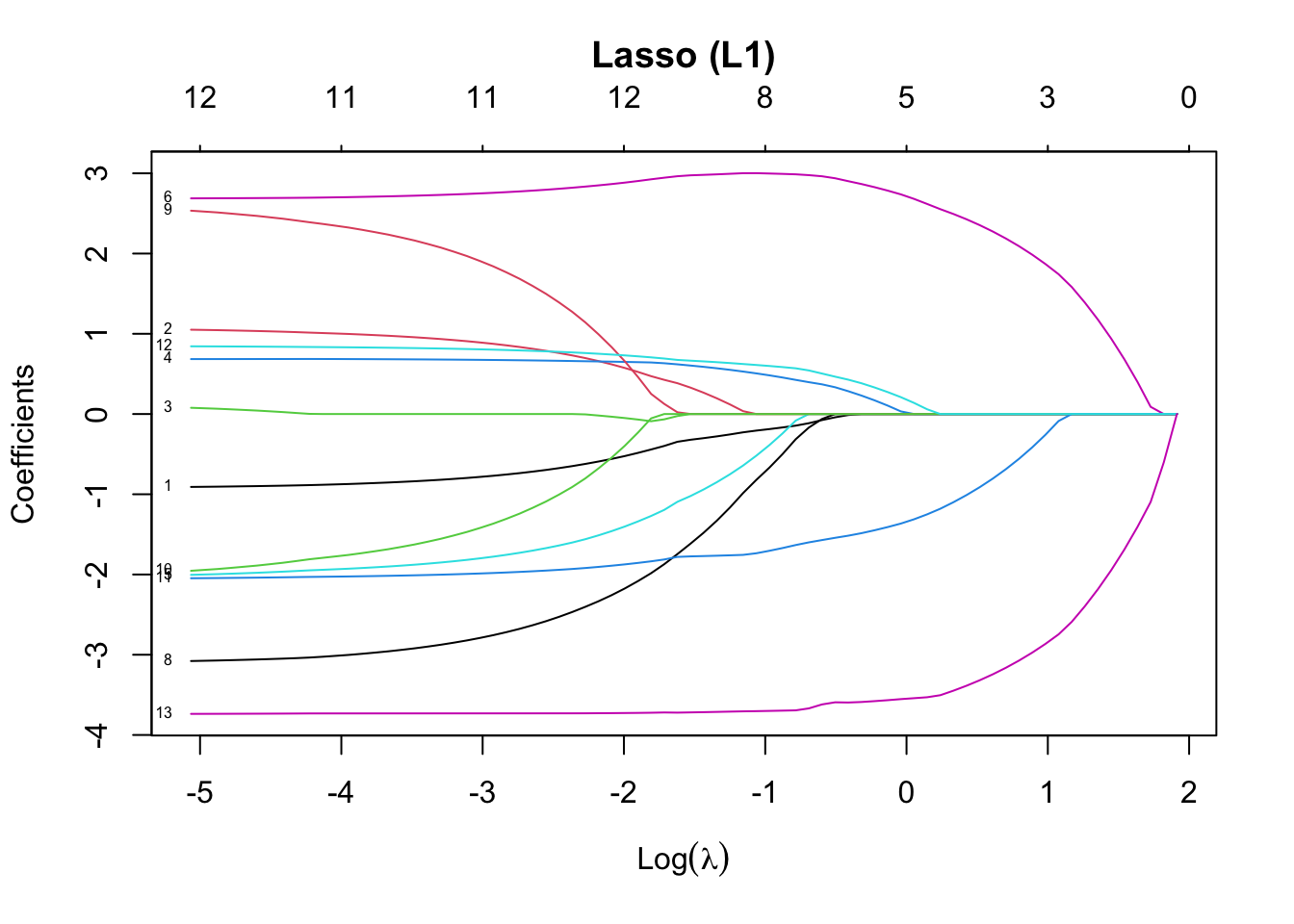
The glmnet::plot() function displays how coefficients change with different levels of regularization (λ). By plotting Ridge (L2) and Lasso (L1) side by side:
- You’ll see L2 (Ridge) smoothly shrinks all coefficients
- You’ll see L1 (Lasso) drops many coefficients to exactly zero — useful for feature selection
This visual comparison reinforces the intuition behind both techniques.
18.2 R Code
library(tidyverse)
library(glmnet)
library(patchwork)  # For side-by-side plots

# Load and prepare data
df <- read_csv("data/boston_housing.csv")
X <- df %>% select(-medv)
y <- df$medv

# Standardize predictors
X_scaled <- scale(as.matrix(X))
y_vec <- as.numeric(y)

# Fit Ridge (alpha = 0) and Lasso (alpha = 1)
ridge_model <- glmnet(X_scaled, y_vec, alpha = 0)
lasso_model <- glmnet(X_scaled, y_vec, alpha = 1)

# Plot both with patchwork
plot_ridge <- plot(ridge_model, xvar = "lambda", label = TRUE, main = "Ridge (L2)\n") 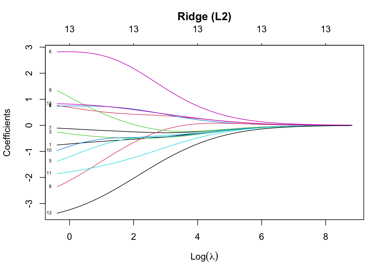
# Display side by side (patchwork wraps ggplots; glmnet plots use base)
# So we use layout to show the effect — OR plot in sequence with par(mfrow)
par(mfrow = c(1, 2))  # Base R layout
plot(ridge_model, xvar = "lambda", label = TRUE, main = "Ridge (L2)\n")
plot(lasso_model, xvar = "lambda", label = TRUE, main = "Lasso (L1)\n")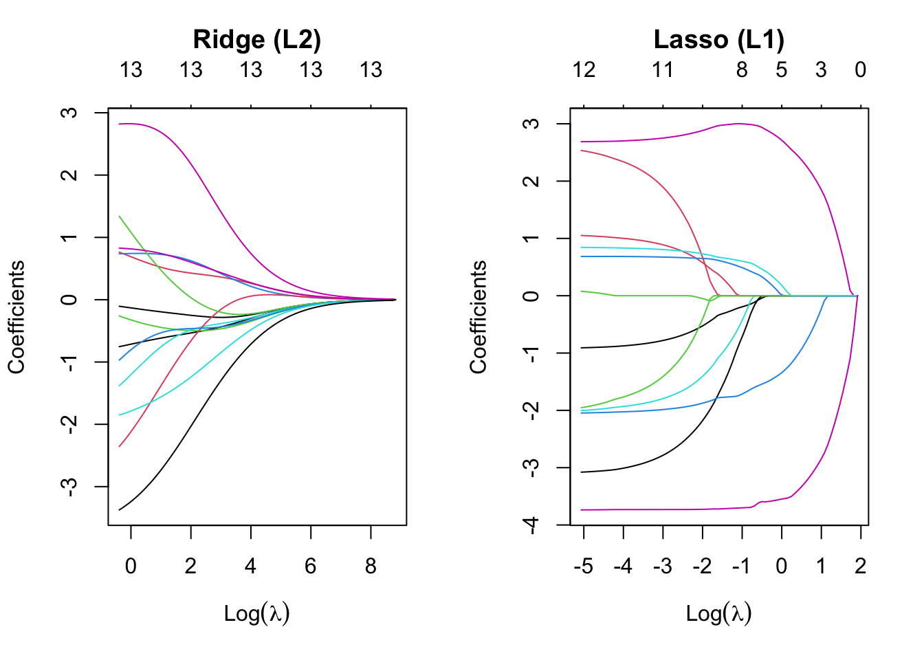
✅ Takeaway: Ridge regularization shrinks all coefficients but keeps them nonzero. Lasso can reduce some coefficients to exactly zero — making it a natural tool for feature selection.