Q&A 28 How do you explain predictions using SHAP or LIME?

28.1 Explanation

After training a machine learning model, interpreting its predictions is crucial for trust, fairness, and debugging. Two powerful, model-agnostic tools used for interpretation are:

• SHAP (SHapley Additive exPlanations): Based on game theory; assigns each feature an importance value for a particular prediction.
• LIME (Local Interpretable Model-agnostic Explanations): Approximates the model locally by fitting a simpler interpretable model near the prediction of interest.

Both help answer: “Which features contributed to this prediction and how?”

---

28.2 Python Code

import pandas as pd
import shap
import lime
import lime.lime_tabular
from sklearn.ensemble import RandomForestRegressor
from sklearn.model_selection import train_test_split
from sklearn.preprocessing import StandardScaler

# Load dataset
df = pd.read_csv("data/boston_housing.csv")
X = df.drop("medv", axis=1)
y = df["medv"]

# Train-test split
X_train, X_test, y_train, y_test = train_test_split(X, y, test_size=0.2, random_state=42)

# Train model
model = RandomForestRegressor(n_estimators=100, random_state=42)
model.fit(X_train, y_train)

RandomForestRegressor(random_state=42)

In a Jupyter environment, please rerun this cell to show the HTML representation or trust the notebook.
On GitHub, the HTML representation is unable to render, please try loading this page with nbviewer.org.

# --- SHAP ---
explainer = shap.Explainer(model.predict, X_train)
shap_values = explainer(X_test[:50])

# Visualize SHAP values
shap.plots.beeswarm(shap_values)

PermutationExplainer explainer: 82%|███████████████████████████████████▎ | 41/50 [00:00<?, ?it/s]

PermutationExplainer explainer: 86%|██████████████████████████████ | 43/50 [00:10<00:00, 10.51it/s]

PermutationExplainer explainer: 90%|███████████████████████████████▌ | 45/50 [00:10<00:00, 6.52it/s]

PermutationExplainer explainer: 92%|████████████████████████████████▏ | 46/50 [00:10<00:00, 5.90it/s]

PermutationExplainer explainer: 94%|████████████████████████████████▉ | 47/50 [00:11<00:00, 5.72it/s]

PermutationExplainer explainer: 96%|█████████████████████████████████▌ | 48/50 [00:11<00:00, 5.56it/s]

PermutationExplainer explainer: 98%|██████████████████████████████████▎| 49/50 [00:11<00:00, 5.37it/s]

PermutationExplainer explainer: 100%|███████████████████████████████████| 50/50 [00:11<00:00, 5.31it/s]

PermutationExplainer explainer: 51it [00:11, 5.27it/s]

PermutationExplainer explainer: 51it [00:11, 1.18s/it]

# --- LIME ---
explainer_lime = lime.lime_tabular.LimeTabularExplainer(
    training_data=X_train.values,
    feature_names=X_train.columns.tolist(),
    mode='regression'
)

# Explain a single prediction
i = 1
exp = explainer_lime.explain_instance(X_test.iloc[i].to_numpy(), lambda x: model.predict(pd.DataFrame(x, columns=X_test.columns)))
exp.show_in_notebook()

28.3 R Coce

library(iml)
library(DALEX)
library(randomForest)
library(readr)

# Load and prepare data
df <- read_csv("data/boston_housing.csv")
df <- df[complete.cases(df), ]
X <- df[, setdiff(names(df), "medv")]
y <- df$medv

# Train model
rf_model <- randomForest(X, y, ntree = 100)

# --- DALEX ---
explainer <- explain(
  model = rf_model,
  data = X,
  y = y,
  label = "Random Forest"
)

Preparation of a new explainer is initiated
  -> model label       :  Random Forest 
  -> data              :  506  rows  13  cols 
  -> data              :  tibble converted into a data.frame 
  -> target variable   :  506  values 
  -> predict function  :  yhat.randomForest  will be used (  default  )
  -> predicted values  :  No value for predict function target column. (  default  )
  -> model_info        :  package randomForest , ver. 4.7.1.2 , task regression (  default  ) 
  -> predicted values  :  numerical, min =  6.466105 , mean =  22.54425 , max =  49.00127  
  -> residual function :  difference between y and yhat (  default  )
  -> residuals         :  numerical, min =  -5.101683 , mean =  -0.01144526 , max =  11.37555  
  A new explainer has been created!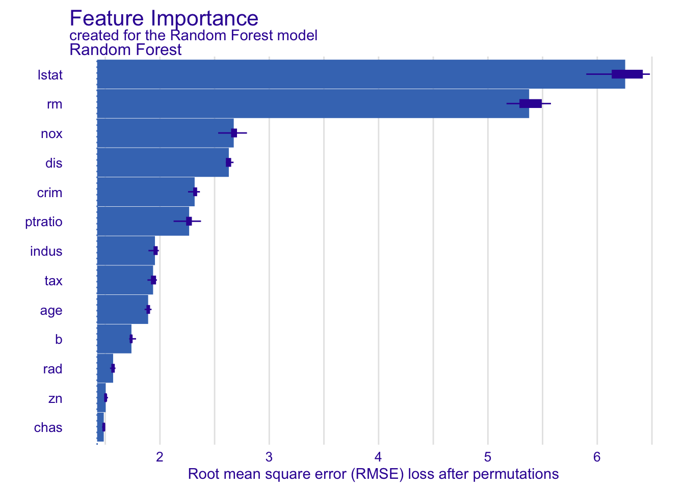  

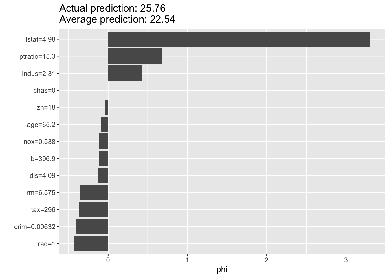
# Feature importance
fi <- model_parts(explainer)
plot(fi)

# --- IML for SHAP ---
predictor <- Predictor$new(rf_model, data = X, y = y)
shap <- Shapley$new(predictor, x.interest = X[1, ])
plot(shap)