Q&A 11 How do you train a random forest model and check variable importance?

11.1 Explanation

A Random Forest is an ensemble model made of many decision trees. It improves performance and reduces overfitting by averaging the results of multiple trees trained on random subsets of the data and features.

One of its strengths is the ability to estimate feature importance, showing which variables most influence predictions.

---

11.2 Python Code

# Train a Random Forest model in Python
import pandas as pd
from sklearn.model_selection import train_test_split
from sklearn.ensemble import RandomForestClassifier
from sklearn.metrics import accuracy_score
import matplotlib.pyplot as plt

# Load and preprocess
df = pd.read_csv("data/titanic.csv")
df['Age'] = df['Age'].fillna(df['Age'].median())
df['Embarked'] = df['Embarked'].fillna(df['Embarked'].mode()[0])
df['Sex'] = df['Sex'].map({'male': 0, 'female': 1})
df = pd.get_dummies(df, columns=['Embarked'], drop_first=True)

# Features and target
X = df[['Pclass', 'Sex', 'Age', 'Fare', 'Embarked_Q', 'Embarked_S']]
y = df['Survived']

# Split
X_train, X_test, y_train, y_test = train_test_split(X, y, test_size=0.2, random_state=42)

# Train Random Forest
rf_model = RandomForestClassifier(n_estimators=100, random_state=42)
rf_model.fit(X_train, y_train)

# Predict and evaluate
y_pred = rf_model.predict(X_test)
print("Accuracy:", accuracy_score(y_test, y_pred))

# Plot feature importance
importances = rf_model.feature_importances_
features = X.columns
plt.barh(features, importances)
plt.xlabel("Feature Importance")
plt.title("Random Forest - Feature Importance")
plt.show()

Accuracy: 0.7932960893854749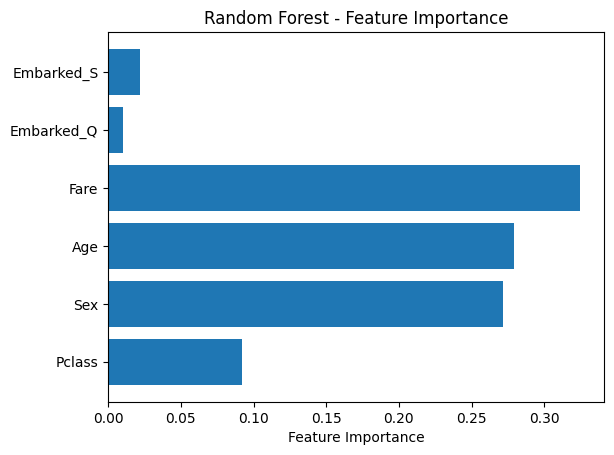

11.3 R Code

# Train a Random Forest model in R and check variable importance
library(readr)
library(dplyr)
library(fastDummies)
library(caret)
library(randomForest)

# Load and preprocess
df <- read_csv("data/titanic.csv")
df$Age[is.na(df$Age)] <- median(df$Age, na.rm = TRUE)
mode_embarked <- names(sort(table(df$Embarked), decreasing = TRUE))[1]
df$Embarked[is.na(df$Embarked)] <- mode_embarked
df$Sex <- ifelse(df$Sex == "male", 0, 1)
df <- fastDummies::dummy_cols(df, select_columns = "Embarked", remove_first_dummy = TRUE, remove_selected_columns = TRUE)

# Feature and target
features <- df %>% select(Pclass, Sex, Age, Fare, Embarked_Q, Embarked_S)
target <- df$Survived

# Split
set.seed(42)
split_index <- createDataPartition(target, p = 0.8, list = FALSE)
X_train <- features[split_index, ]
X_test <- features[-split_index, ]
y_train <- target[split_index]
y_test <- target[-split_index]

# Train Random Forest
rf_model <- randomForest(x = X_train, y = as.factor(y_train), ntree = 100, importance = TRUE)

# Predict and evaluate
y_pred <- predict(rf_model, X_test)
confusionMatrix(y_pred, as.factor(y_test))

Confusion Matrix and Statistics

          Reference
Prediction   0   1
         0 104  25
         1  10  39
                                          
               Accuracy : 0.8034          
                 95% CI : (0.7373, 0.8591)
    No Information Rate : 0.6404          
    P-Value [Acc > NIR] : 1.629e-06       
                                          
                  Kappa : 0.5499          
                                          
 Mcnemar's Test P-Value : 0.01796         
                                          
            Sensitivity : 0.9123          
            Specificity : 0.6094          
         Pos Pred Value : 0.8062          
         Neg Pred Value : 0.7959          
             Prevalence : 0.6404          
         Detection Rate : 0.5843          
   Detection Prevalence : 0.7247          
      Balanced Accuracy : 0.7608          
                                          
       'Positive' Class : 0               
                                          

# Plot feature importance
varImpPlot(rf_model)

✅ Takeaway: Random forests combine accuracy with interpretability. They’re a go-to choice when you want a strong baseline and a clear view of which features drive predictions.