Q&A 8 How do you evaluate model performance using a confusion matrix and accuracy?

8.1 Explanation

Once a classification model is trained, it’s important to evaluate how well it performs on unseen data. Two common tools are:

• Confusion Matrix: Shows the number of correct and incorrect predictions categorized by actual vs. predicted labels.
• Accuracy: The ratio of correct predictions to total predictions.

These metrics help you understand whether your model is truly learning or just guessing.

---

8.2 Python Code

# Evaluate classification model in Python
import pandas as pd
from sklearn.model_selection import train_test_split
from sklearn.tree import DecisionTreeClassifier
from sklearn.metrics import accuracy_score, confusion_matrix, ConfusionMatrixDisplay

# Load and preprocess the data
df = pd.read_csv("data/titanic.csv")
df['Age'] = df['Age'].fillna(df['Age'].median())
df['Embarked'] = df['Embarked'].fillna(df['Embarked'].mode()[0])
df['Sex'] = df['Sex'].map({'male': 0, 'female': 1})
df = pd.get_dummies(df, columns=['Embarked'], drop_first=True)

# Feature set and labels
X = df[['Pclass', 'Sex', 'Age', 'Fare', 'Embarked_Q', 'Embarked_S']]
y = df['Survived']

# Split data
X_train, X_test, y_train, y_test = train_test_split(X, y, test_size=0.2, random_state=42)

# Train model
clf = DecisionTreeClassifier(random_state=42)
clf.fit(X_train, y_train)
y_pred = clf.predict(X_test)

# Accuracy
print("Accuracy:", accuracy_score(y_test, y_pred))

# Confusion Matrix
cm = confusion_matrix(y_test, y_pred)
print("Confusion Matrix:\n", cm)

# Visualize Confusion Matrix
disp = ConfusionMatrixDisplay(confusion_matrix=cm, display_labels=clf.classes_)
disp.plot()

Accuracy: 0.7877094972067039
Confusion Matrix:
 [[84 21]
 [17 57]]





<sklearn.metrics._plot.confusion_matrix.ConfusionMatrixDisplay at 0x14e5f7260>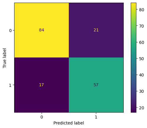

# Evaluate classification model in R
library(readr)
library(dplyr)
library(fastDummies)
library(caret)
library(rpart)
library(ggplot2)
library(reshape2)

# Load and preprocess
df <- read_csv("data/titanic.csv", show_col_types = FALSE)
df$Age[is.na(df$Age)] <- median(df$Age, na.rm = TRUE)
mode_embarked <- names(sort(table(df$Embarked), decreasing = TRUE))[1]
df$Embarked[is.na(df$Embarked)] <- mode_embarked
df$Sex <- ifelse(df$Sex == "male", 0, 1)
df <- fastDummies::dummy_cols(df, select_columns = "Embarked", remove_first_dummy = TRUE, remove_selected_columns = TRUE)

# Split and train
features <- df %>% select(Pclass, Sex, Age, Fare, Embarked_Q, Embarked_S)
target <- df$Survived
set.seed(42)
split_index <- createDataPartition(target, p = 0.8, list = FALSE)
X_train <- features[split_index, ]
X_test <- features[-split_index, ]
y_train <- target[split_index]
y_test <- target[-split_index]
train_data <- cbind(X_train, Survived = y_train)
tree_model <- rpart(Survived ~ ., data = train_data, method = "class")
y_pred <- predict(tree_model, X_test, type = "class")

# Evaluate performance
confusion <- confusionMatrix(y_pred, as.factor(y_test))
print(confusion$table)

          Reference
Prediction   0   1
         0 101  25
         1  13  39

# Get confusion matrix as a table
conf_matrix <- confusionMatrix(y_pred, as.factor(y_test))
cm_table <- as.table(conf_matrix$table)

# Convert to dataframe for plotting
cm_df <- as.data.frame(cm_table)
colnames(cm_df) <- c("Prediction", "Reference", "Freq")

# Plot heatmap
ggplot(data = cm_df, aes(x = Reference, y = Prediction, fill = Freq)) +
  geom_tile(color = "white") +
  geom_text(aes(label = Freq), vjust = 0.5, size = 5) +
  scale_fill_gradient(low = "yellow", high = "skyblue") +
  labs(title = "Confusion Matrix", x = "Actual", y = "Predicted") +
  theme_minimal()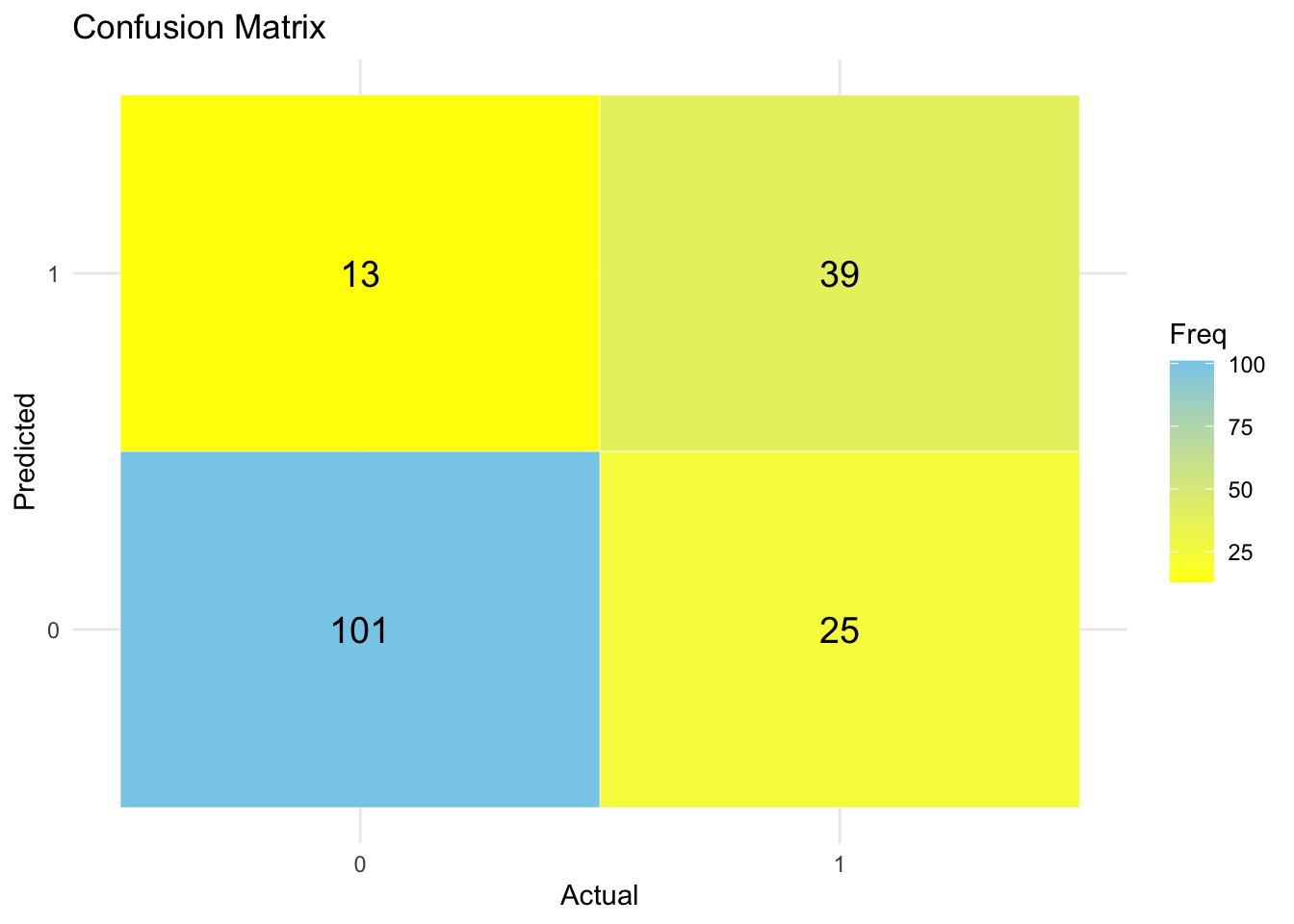

✅ Takeaway: A confusion matrix provides a full picture of your model’s performance — not just how often it’s right, but also how and where it makes mistakes. Always pair it with accuracy to evaluate your model meaningfully.