Q&A 26 How do you create a heatmap to compare model performance across metrics?

26.1 Explanation

Once you’ve trained multiple models, comparing their performance across multiple metrics — like accuracy, precision, recall, F1-score, and AUC — provides a deeper understanding of their strengths and weaknesses.

Instead of viewing one metric at a time, a heatmap helps summarize all key metrics in one chart, allowing for quicker and more informed decisions when choosing a model.

---

26.2 Python Code

# Compare models using performance metrics heatmap (Python) — safe version
import pandas as pd
import seaborn as sns
import matplotlib.pyplot as plt
from sklearn.metrics import accuracy_score, precision_score, recall_score, f1_score, roc_auc_score
from sklearn.model_selection import train_test_split
from sklearn.preprocessing import LabelEncoder
from sklearn.linear_model import LogisticRegression
from sklearn.ensemble import RandomForestClassifier
from sklearn.svm import SVC
from sklearn.naive_bayes import GaussianNB

# Load and prepare Titanic data
df = pd.read_csv("data/titanic.csv")
df = df.dropna(subset=["Age", "Fare", "Embarked", "Sex", "Survived"])

# Make a copy to avoid SettingWithCopyWarning
X = df[["Pclass", "Age", "Fare"]].copy()

# Encode categorical variables safely using .loc
X.loc[:, "Sex"] = LabelEncoder().fit_transform(df["Sex"])
X.loc[:, "Embarked"] = LabelEncoder().fit_transform(df["Embarked"])
y = df["Survived"]

# Train-test split
X_train, X_test, y_train, y_test = train_test_split(X, y, test_size=0.3, random_state=42)

# Models to compare
models = {
    "LogReg": LogisticRegression(solver="liblinear"),
    "RandomForest": RandomForestClassifier(n_estimators=100, random_state=42),
    "SVM": SVC(probability=True, gamma="auto", random_state=42),
    "NaiveBayes": GaussianNB()
}

# Evaluate and collect metrics
metrics_list = []

for name, model in models.items():
    model.fit(X_train, y_train)
    y_pred = model.predict(X_test)
    y_prob = model.predict_proba(X_test)[:, 1]

    metrics_list.append({
        "Model": name,
        "Accuracy": accuracy_score(y_test, y_pred),
        "Precision": precision_score(y_test, y_pred),
        "Recall": recall_score(y_test, y_pred),
        "F1": f1_score(y_test, y_pred),
        "AUC": roc_auc_score(y_test, y_prob)
    })

# Create DataFrame from metrics
metrics_df = pd.DataFrame(metrics_list).set_index("Model")

# Plot heatmap
plt.figure(figsize=(8, 5))
sns.heatmap(metrics_df, annot=True, fmt=".2f", cmap="YlGnBu")
plt.title("Model Performance Comparison")
plt.tight_layout()
plt.show()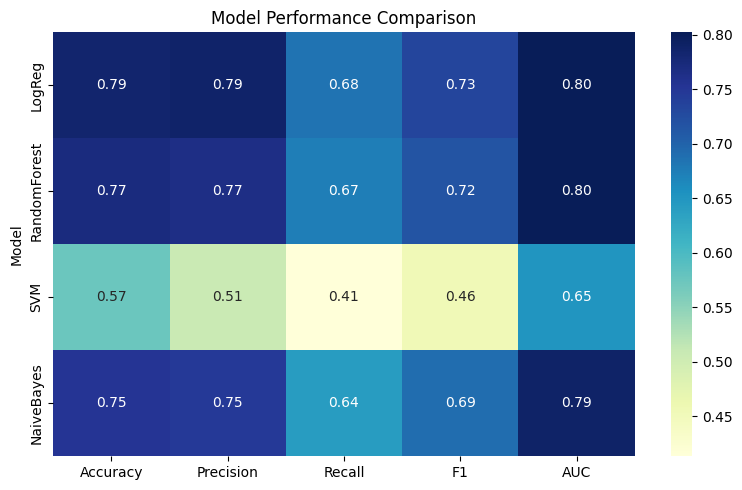

26.3 R Code

# Compare models using performance metrics heatmap (R)
library(readr)
library(dplyr)
library(tidyr)
library(caret)
library(pROC)
library(ggplot2)
library(reshape2)

# Load Titanic dataset
df <- read_csv("data/titanic.csv") %>%
  drop_na(Age, Fare, Embarked, Sex, Survived)

# Prepare data
df <- df %>%
  mutate(
    Sex = as.factor(Sex),
    Embarked = as.factor(Embarked),
    Survived = as.factor(Survived)
  )

# Features and labels
X <- df %>% dplyr::select(Pclass, Age, Fare, Sex, Embarked)
y <- df$Survived

# Train-test split
set.seed(42)
train_index <- createDataPartition(y, p = 0.7, list = FALSE)
train_data <- df[train_index, ]
test_data  <- df[-train_index, ]


# Define formula with only clean columns
ml_formula <- Survived ~ Pclass + Age + Fare + Sex + Embarked

# Train models safely
models <- list(
  LogReg = train(ml_formula, data = train_data, method = "glm", family = "binomial"),
  RandomForest = train(ml_formula, data = train_data, method = "rf"),
  SVM = train(ml_formula, data = train_data, method = "svmRadial"),
  NaiveBayes = train(ml_formula, data = train_data, method = "naive_bayes")
)

# Metric evaluation function
get_metrics <- function(model, test_data) {
  pred <- predict(model, test_data)
  prob_df <- tryCatch({
    predict(model, test_data, type = "prob")
  }, error = function(e) {
    warning(paste("Skipping prob for model due to:", e$message))
    return(NULL)
  })

  obs <- test_data$Survived

  if (!is.null(prob_df) && "Yes" %in% colnames(prob_df)) {
    prob <- prob_df[["Yes"]]
    auc_val <- tryCatch({
      roc(obs, prob)$auc
    }, error = function(e) {
      warning(paste("AUC failed for model due to:", e$message))
      return(NA)
    })
  } else {
    prob <- rep(NA, length(obs))
    auc_val <- NA
  }

  data.frame(
    Accuracy  = mean(pred == obs),
    Precision = tryCatch(posPredValue(pred, obs, positive = "Yes"), error = function(e) NA),
    Recall    = tryCatch(sensitivity(pred, obs, positive = "Yes"), error = function(e) NA),
    F1        = tryCatch(F_meas(pred, obs, positive = "Yes"), error = function(e) NA),
    AUC       = auc_val
  )
}

# Collect all model metrics
metric_list <- lapply(models, get_metrics, test_data = test_data)
metric_df <- bind_rows(metric_list, .id = "Model")

# Plot heatmap
metric_long <- melt(metric_df, id.vars = "Model")

ggplot(metric_long, aes(x = variable, y = Model, fill = value)) +
  geom_tile(color = "white") +
  geom_text(aes(label = sprintf("%.2f", value)), size = 3) +
  scale_fill_gradient(low = "yellow", high = "red") +
  labs(title = "Model Performance Comparison", x = "Metric", y = "Model") +
  theme_minimal()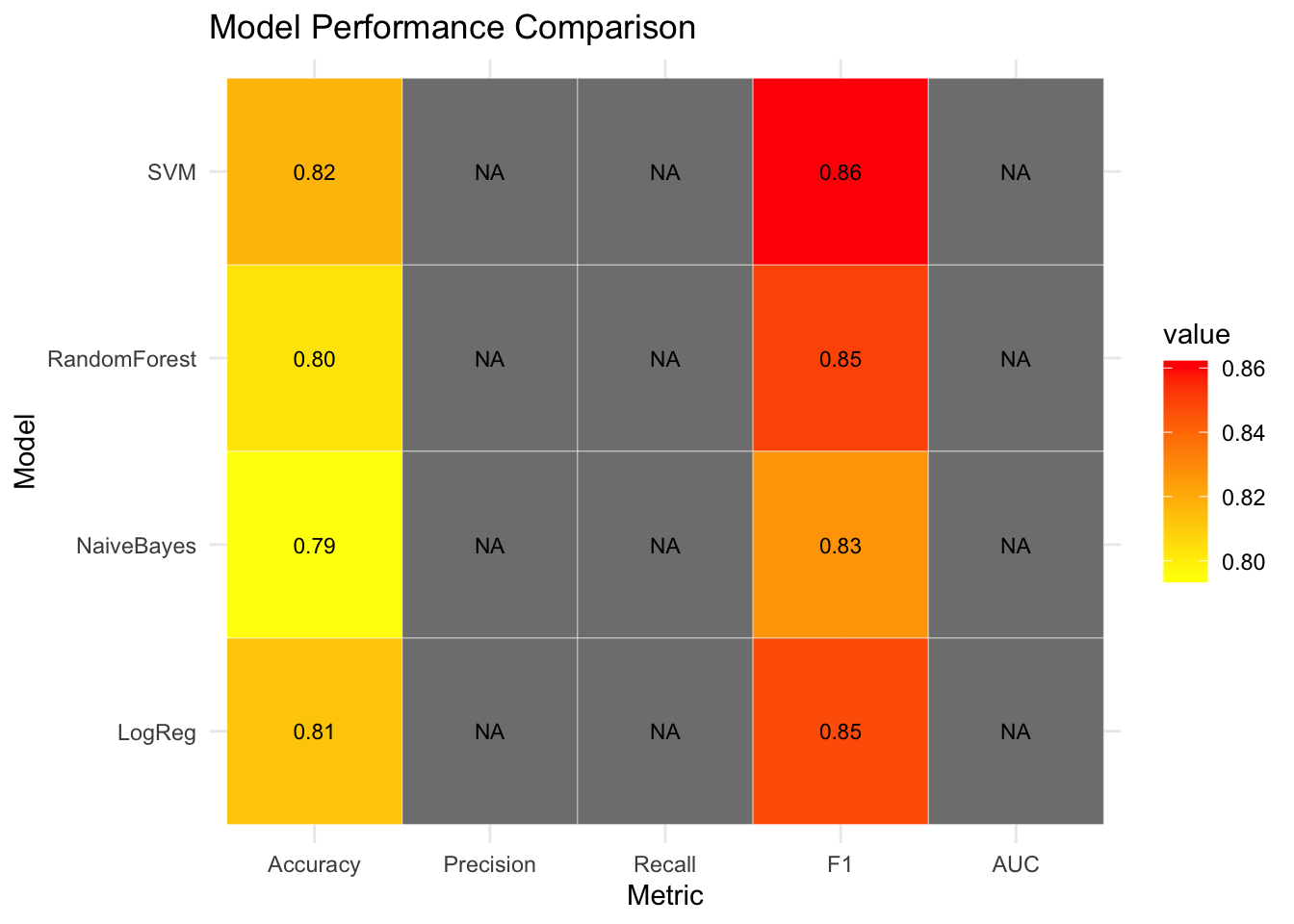

✅ Takeaway: Comparing multiple models in one place lets you make evidence-based decisions — not just based on accuracy, but also on precision, recall, F1, and AUC. A heatmap helps visually spot strengths and weaknesses across classifiers.